Getting Started with MBNpy

This guide intorudces using MBNpy for risk/reliability analysis of system event. This guide walks through installation, defining variables and probability distributions, and performing system analysis.

---

Installation

MBNpy is available via pip:

pip install mbnpy

To install from source:

git clone https://github.com/jieunbyun/MBNpy.git
cd MBNpy
pip install .

MBNpy requires Python 3.12+.

---

Example Problem

This example demonstrates application for the reliability block diagram from the 2019 MBN paper.

The system consists of 8 components (\(X1\) to \(X8\)), each with two states:

• \(0\): Failure

• \(1\): Survival

Components are statistically independent with:

• \(P(X_i=0) = 0.1\)

• \(P(X_i=1) = 0.9\)

The system state (:math:`X_9`) depends on the connection from source to sink.

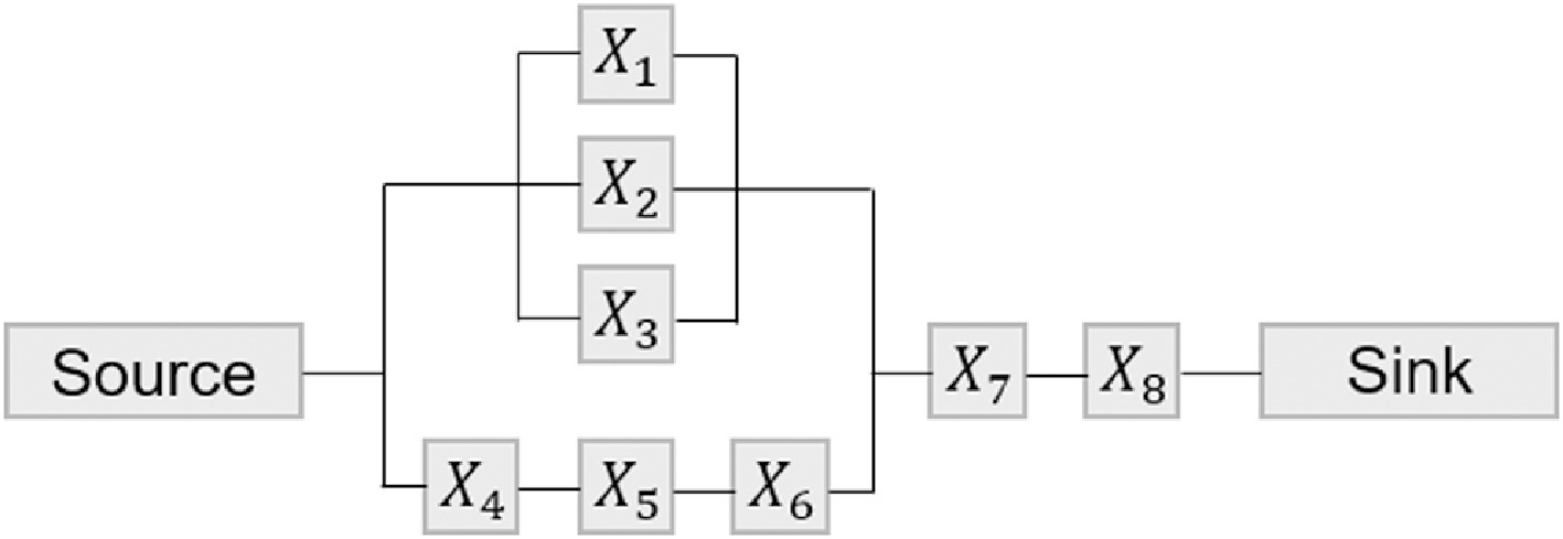
Figure 1: Reliability block diagram (RBD).

The Bayesian network (BN) representation is:

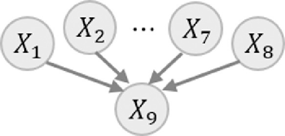
Figure 2: Bayesian network representation of the system.

---

Objectives

1. Compute the system failure probability \(P(X_9=0)\).

2. Identify critical components using component importance measures.

For technical details, see:

Byun et al. (2019) Matrix-based Bayesian networks, Reliability Engineering & System Safety, 185, 533-545.

Byun & Song (2021) Generalized matrix-based Bayesian networks, Reliability Engineering & System Safety, 211, 107468.

---

Defining Variables in MBNpy

To model a Bayesian network, variables must be defined first.

Each component is a Variable object:

from mbnpy import variable

varis = {}
varis['x1'] = variable.Variable(name='x1', values=['f', 's'])

• The variable dictionary (varis) stores all model variables.

• "f" and "s" correspond to failure (0) and survival (1).

• The numerical index assigned to each state is determined by its position in the values list.

All 8 components are defined using a loop:

n_comp = 8
for i in range(1, n_comp):
    varis[f'x{i+1}'] = variable.Variable(name=f'x{i+1}', values=['f', 's'])

print(varis['x8'])  # Check last component

The system variable (\(X_9\)) is defined similarly:

varis['x9'] = variable.Variable(name='x9', values=['f', 's'])

---

Defining Probability Distributions

The conditional probability matrix (CPM) represents probability distributions.

Since components (\(X_1\) to \(X_8\)) have no parents, they are defined as marginal probabilities:

from mbnpy import cpm
import numpy as np

cpms = {}
cpms['x1'] = cpm.Cpm(
    variables=[varis['x1']],
    no_child=1,
    C=np.array([[0], [1]]),
    p=np.array([0.1, 0.9])
)

• variables: A list of variables involved in the distribution (e.g., X1).

• no_child: The number of child nodes (1 in this case).

• C (Event Matrix): Specifies the state of each instance.

• p (Probability Vector): Defines the corresponding probabilities.

This process is repeated for all components:

for i in range(1, n_comp):
    cpms[f'x{i+1}'] = cpm.Cpm(
        variables=[varis[f'x{i+1}']],
        no_child=1,
        C=np.array([[0], [1]]),
        p=np.array([0.1, 0.9])
    )

The system (\(X_9\)) is defined using the branch-and-bound method:

The Csys and psys matrices are constructed (for more information about building C matrices, see composite state tutorial <https://jieunbyun.github.io/MBNpy-docs/composite_states>_):

Csys = np.array([
    [0, 2, 2, 2, 2, 2, 2, 2, 0],
    [0, 2, 2, 2, 2, 2, 2, 0, 1],
    [1, 1, 2, 2, 2, 2, 2, 1, 1],
    [1, 0, 1, 2, 2, 2, 2, 1, 1],
    [1, 0, 0, 1, 2, 2, 2, 1, 1],
    [0, 0, 0, 0, 0, 2, 2, 1, 1],
    [0, 0, 0, 0, 1, 0, 2, 1, 1],
    [0, 0, 0, 0, 1, 1, 0, 1, 1],
    [1, 0, 0, 0, 1, 1, 1, 1, 1]
])
psys = np.array([[1.0] * 9]).T

cpms['x9'] = cpm.Cpm(
    variables=[varis['x9'], varis['x1'], varis['x2'], varis['x3'], varis['x4'],
               varis['x5'], varis['x6'], varis['x7'], varis['x8']],
    no_child=1,
    C=Csys,
    p=psys
)

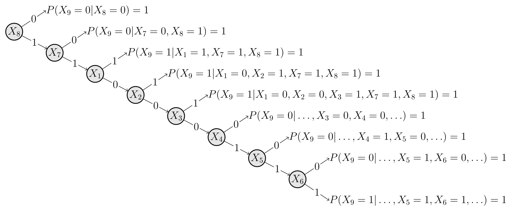
Notes on the branch-and-bound methods and building CPMs

• Each branch forms a row in the CPM for \(P(X_9|X_1, \ldots, X_8)\), where the nine branches lead to the nine rows in Csys and psys.

  For example, Csys’s first row represents the top branch: [0, 2, 2, 2, 2, 2, 2, 2, 0] indicates that if \(X_8=0\), then \(X_9=0\).

  The probabilistic relation \(P(X_9=0|X_8=0) = 1\) is represented in psys as 1.0.

• For deterministic systems whose state is fully determined by their components’ states (which is the case here), the probability vector p contains only 1.0 values.

• The composite state 2 in the event matrix C denotes a “don’t care” condition (i.e. it can represent the state of either 0 or 1), meaning that the corresponding component’s state does not affect the outcome.

  For example, in the first row of Csys, all components except \(X_8\) are marked as 2, indicating that their states do not influence the system state when \(X_8=0\).

• The most important constraint when building a CPM is that the rows in the event matrix C must be mutually exclusive so that no instances are double-counted. The branch-and-bound method ensures this condition is met.

  For example, since the first row of Csys already accounts for all cases where \(X_8=0\), the second row only needs to consider cases where \(X_8=1\).

• For general systems, manual construction of branch-and-bound trees often becomes infeasible.

  In such cases, the BRC algorithm can be used to automatically build a branch-and-bound tree and thereby construct the CPM.

---

System Analysis

Variable elimination is applied to compute the system failure probability. To determine the probability distribution of the system event, all component variables except for \(X_9\) are eliminated.

Note that the second argument of the variable_elim function is a list of variables to eliminate, in the order they should be eliminated.

from mbnpy import inference

# Compute P(X_9) by eliminating all component variables
cpm_sys = inference.variable_elim(
    cpms = cpms, var_elim = [varis['x1'], varis['x2'], varis['x3'], varis['x4'], varis['x5'], varis['x6'], varis['x7'], varis['x8']]
)

# Get probability P(X_9=0) from the resulting CPM
prob_s0 = cpm_sys.get_prob(['x9'], [0])
print(f'System failure probability P(X9=0): {prob_s0:.2f}')

Component importance measures are calculated, following Kang et al. (2008)’s definition \(CIM_i = P(X_i=0|X_9=0) = P(X_i=0,X_9=0) / P(X_9=0)\):

CIMs = {}
for i in range(n_comp):

    # Current component of interest
    var_i = f'x{i+1}'

    # Variables to eliminate: all except the component of interest and the system variable
    varis_elim = [varis['x1'], varis['x2'], varis['x3'], varis['x4'], varis['x5'], varis['x6'], varis['x7'], varis['x8']]
    varis_elim.remove(varis[var_i])

    # Compute P(X_i, X_9)
    cpm_sys_xi = inference.variable_elim(cpms = cpms, var_elim = varis_elim)
    # Get probability P(X_i=0, X_9=0) from the resulting CPM
    prob_s0_x0 = cpm_sys_xi.get_prob([f'x{i+1}', 'x9'], [0,0])

    # Compute CIM_i = P(X_i=0|X_9=0) = P(X_i=0, X_9=0) / P(X_9=0)
    CIMs[f'x{i+1}'] = prob_s0_x0 / prob_s0 # prob_s0 represents P(X_9=0), from the previous computation

print(CIMs)