Getting Started with the BRC Algorithm
Note
The Branch and Bound Algorithm for Reliability of Coherent Systems (BRC) is an efficient method for analysing system reliability with discrete-state component events and a binary-state system event. It identifies (sub-)minimal survival and failure rules while computing system failure probability using a branch-and-bound approach. Official publication is available at arXiv.
Introduction
The BRC algorithm identifies (sub-)minimal survival and failure rules and computes the system failure probability using a branch-and-bound approach.
BRC applies to any general coherent system, meaning systems where an improvement in component states never leads to a worse system state.
The figure below illustrates the BRC process (or more details, refer to the official publication on arXiv):
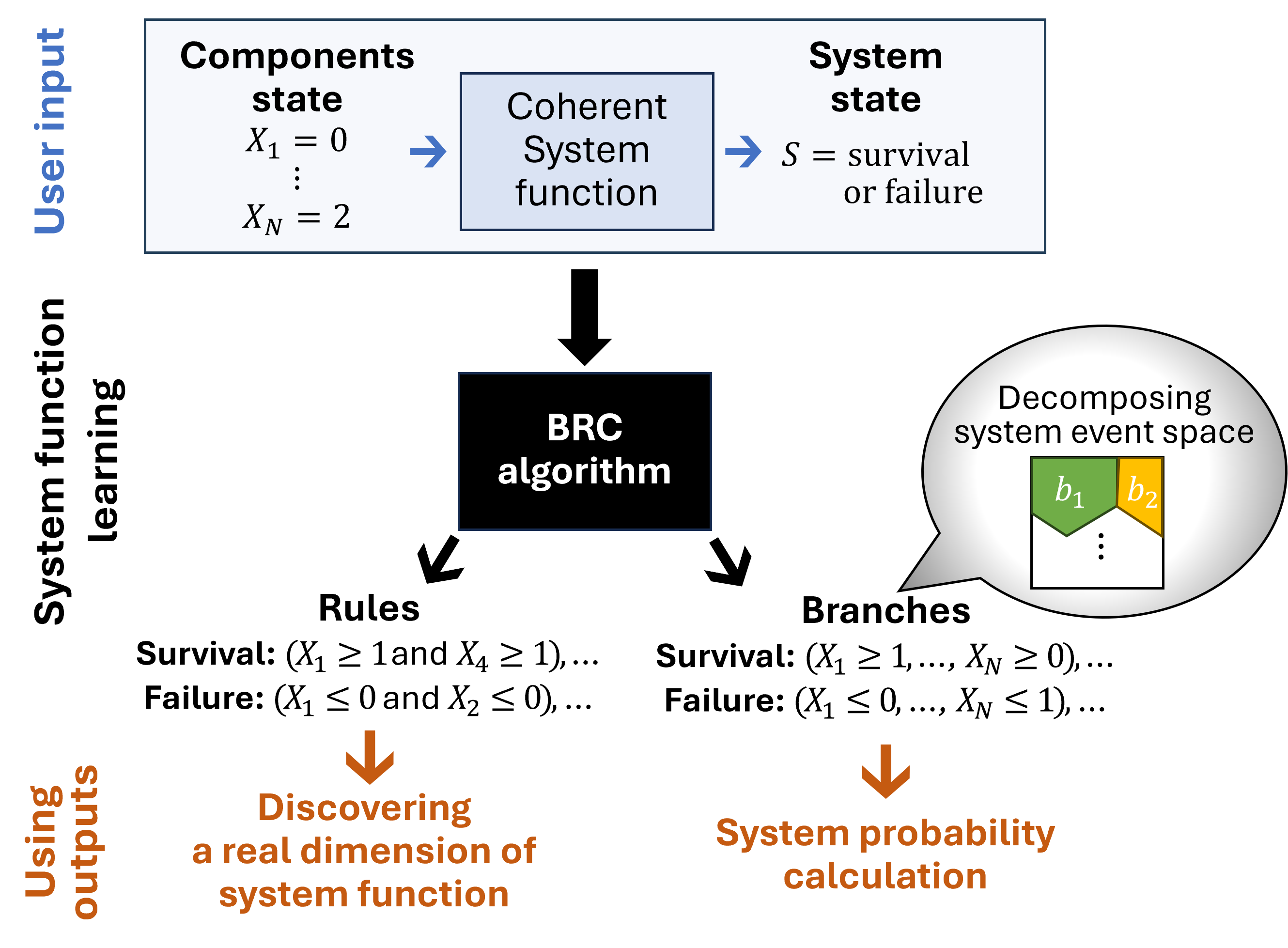
Illustration of the BRC algorithm.
Code Demonstration
The Jupyter notebook for this tutorial is available on GitHub.
MBNPy Version
This tutorial uses MBNPy v0.1.2.
Installation
Ensure you have the required dependencies installed before running the tutorial:
import networkx as nx
import matplotlib.pyplot as plt
from mbnpy import cpm, variable, inference
from networkx.algorithms.flow import shortest_augmenting_path
from mbnpy import brc
import numpy as np
Example: Five-Edge Network
Network Topology
We analyse the five-edge network below:
nodes = {'n1': (0, 0),
         'n2': (1, 1),
         'n3': (1, -1),
         'n4': (2, 0)}

edges = {'e1': ['n1', 'n2'],
         'e2': ['n1', 'n3'],
         'e3': ['n2', 'n3'],
         'e4': ['n2', 'n4'],
         'e5': ['n3', 'n4']}

# Plot network
plt.figure(figsize=(4,3))
G = nx.Graph()
for node in nodes:
    G.add_node(node, pos=nodes[node])
for e, pair in edges.items():
    G.add_edge(*pair, label=e)

pos = nx.get_node_attributes(G, 'pos')
edge_labels=nx.get_edge_attributes(G, 'label')
nx.draw(G, pos, with_labels=True)
nx.draw_networkx_edge_labels(G, pos, edge_labels=edge_labels)
plt.show()
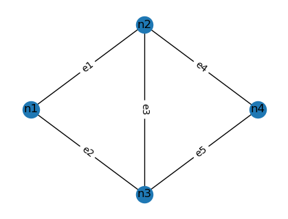
Network topology with five edges.
Defining Component Events
The state of each edge is represented by a binary variable:
varis = {}
for k, v in edges.items():
    varis[k] = variable.Variable(name=k, values=[0, 1])  # 0 = non-functional, 1 = functional

print(varis['e1'])
The probabilities of each component event:
probs = {'e1': {0: 0.01, 1: 0.99},
         'e2': {0: 0.01, 1: 0.99},
         'e3': {0: 0.05, 1: 0.95},
         'e4': {0: 0.05, 1: 0.95},
         'e5': {0: 0.10, 1: 0.90}}
Defining the System Event
The system’s state is determined by connectivity between an origin-destination (OD) pair.
A system function must: - Take a dictionary of component states as input. - Return:
System value (informational).
System state (‘s’ for survival, ‘f’ for failure).
Minimum component state that guarantees the system state.
The function is implemented as follows:
def net_conn(comps_st, od_pair, edges, varis):

    # Build a graph with edge capacities based on component states
    G = nx.Graph()
    for k, st in comps_st.items():
        edge_k = edges[k]
        origin_k, dest_k = edge_k[0], edge_k[1]

        G.add_edge(origin_k, dest_k)

        # Set capacity
        capa_k = varis[k].values[st]  # 1 for functional, 0 for non-functional
        G[origin_k][dest_k]['capacity'] = capa_k

    # To check whether od_pair is connected, as well as the path between them, we add a new edge from destination to a new dummy node with capacity 1 and check if the maximum flow is greater than 0.
    G.add_edge(od_pair[1], 'new_d', capacity=1) # add a dummy edge
    f_val, f_dict = nx.maximum_flow(G, od_pair[0], 'new_d') # compute maximum flow from origin to dummy node

    # Determine the system state and the minimum component state that guarantees the system state
    if f_val > 0: # system survival
        sys_st = 's'
        min_comp_st = {k: 1 for k, x in f_dict.items() if x > 0}  # components with flow > 0 need to be functional for system survival
    else: # system failure
         sys_st = 'f'
         min_comp_st = None  # since it is more complex to determine the minimum component state for system failure, we return None for simplicity

    return f_val, sys_st, min_comp_st # f_val is returned only for informational purposes, and is not used by BRC.
The OD pair is set to (‘n1’, ‘n4’):
od_pair = ('n1', 'n4')
Running the BRC Algorithm
Now, we run the BRC algorithm. By setting the target unknown probability as zero, i.e. pf_bnd_wr=0.0, the analysis terminates after identifying all survival and failure rules:
brs, rules, sys_res, monitor = brc.run(probs, sys_fun, max_sf=np.inf, max_nb=np.inf, pf_bnd_wr=0.0)
When there are many rules, the algorithm can be set to terminate early by setting a positive value for pf_bnd_wr, which is the bound on the probability ratio of unknown branches to failure branches. For example, setting pf_bnd_wr=0.1 terminates the analysis when the probability of unknown probability is less than 10% of that of failure probability.
One can also set a maximum number of rules to generate by setting max_rules. For example, setting max_rules=200 terminates the analysis when 200 rules are generated, regardless of the probability bounds. Emprically, we find BRC struggles to handle more than 200-300 rules, so setting max_rules can be useful for large systems.
BRC output
*** Analysis completed with 8 system function runs ***
System failure probability: 5.16e-3
Found non-dominated rules (failure: 4, survival: 4)
Extracting System Rules
We can check what rules BRC identified:
print(rules['s'])  # Survival rules
print(rules['f'])  # Failure rules
This returns:
Survival Rules: [{'e1': 1, 'e4': 1}, {'e2': 1, 'e5': 1}, {'e2': 1, 'e3': 1, 'e4': 1}, {'e1': 1, 'e3': 1, 'e5': 1}]
Failure Rules: [{'e4': 0, 'e5': 0}, {'e1': 0, 'e2': 0}, {'e1': 0, 'e3': 0, 'e5': 0}, {'e2': 0, 'e3': 0, 'e4': 0}]
It finds four survival and four failure rules. For example, the first survival rule {‘e1’: 1, ‘e4’: 1} indicates that if edges e1 and e4 are functional, then the system survives regardless of the states of other edges.
Setting Up Probability Distributions
BRC branches can be used to construct Conditional Probability Matrices (CPMs) for further probabilistic analysis.
First, we define the system variable and build CPMs for both component and system events:
varis['sys'] = variable.Variable(name='sys', values=['f', 's']) # state 0 for failure and 1 for survival

# probability distributions using CPM
cpms = {}

# component events
for k, v in edges.items():
    cpms[k] = cpm.Cpm( variables = [varis[k]], no_child=1, C = np.array([[0],[1]]), p=np.array([probs[k][0], probs[k][1]]) )

# system event
Csys = branch.get_cmat(branches = brs, comp_varis={'e1': varis['e1'], 'e2': varis['e2'], 'e3': varis['e3'], 'e4': varis['e4'], 'e5': varis['e5']})
print("C matrix of P(sys | e1, e2, e3, e4, e5):")
print(Csys) # each branch becomes a row in the system's event matrix
psys = np.array([1.0]*len(Csys)) # the system function is determinisitic, i.e. all instances have a probability of 1.

# Define CPM of P(sys | e1, e2, e3, e4, e5)
cpms['sys'] = cpm.Cpm( [varis['sys']] + ['e1', 'e2', 'e3', 'e4', 'e5'], 1, Csys, psys )
print(cpms['sys'])
Each branch becomes a row in the system event matrix. Since the system function is deterministic, all probabilities are set to 1:
C matrix of P(sys | e1, e2, e3, e4, e5):
[[1 1 2 2 1 2]
 [1 1 1 2 0 1]
 [1 0 1 1 1 2]
 [0 1 2 2 0 0]
 [0 0 1 1 0 0]
 [1 0 1 1 0 1]
 [0 1 0 0 0 1]
 [1 1 0 1 0 1]
 [1 0 1 0 2 1]
 [0 0 0 2 2 2]
 [0 0 1 0 2 0]]

<CPM representing P(sys | e1, e2, e3, e4, e5)>
+-------+------+------+------+------+------+-----+
|   sys [   e1 |   e2 |   e3 |   e4 |   e5 ]   p |
+=======+======+======+======+======+======+=====+
|     1 [    1 |    2 |    2 |    1 |    2 ]   1 |
+-------+------+------+------+------+------+-----+
|     1 [    1 |    1 |    2 |    0 |    1 ]   1 |
+-------+------+------+------+------+------+-----+
|     1 [    0 |    1 |    1 |    1 |    2 ]   1 |
+-------+------+------+------+------+------+-----+
|     0 [    1 |    2 |    2 |    0 |    0 ]   1 |
+-------+------+------+------+------+------+-----+
|   :   [  :   |  :   |  :   |  :   |  :   ]  :  |
+-------+------+------+------+------+------+-----+
|     1 [    0 |    1 |    0 |    2 |    1 ]   1 |
+-------+------+------+------+------+------+-----+
|     0 [    0 |    0 |    2 |    2 |    2 ]   1 |
+-------+------+------+------+------+------+-----+
|     0 [    0 |    1 |    0 |    2 |    0 ]   1 |
+-------+------+------+------+------+------+-----+
For more information about building C matrices, see composite state tutorial <https://jieunbyun.github.io/MBNpy-docs/composite_states>_.
Computing System Probability
From the CPMs, the system failure probability \(P(S=0)\) can be obtained by variable elimination (cf. MBNpy tutorial):
var_elim_order = ['e1', 'e2', 'e3', 'e4', 'e5']

cpm_s = inference.variable_elim(cpms = cpms, var_elim = var_elim_order)
print(cpm_s)
This returns:
<CPM representing P(sys | )>
+-------+------------+
|   sys [ ]          p |
+=======+============+
|     1 [ ] 0.994831 |
+-------+------------+
|     0 [ ] 0.005169 |
+-------+------------+
The system failure probability is \(P(S=0) = 5.17 \times 10^{-3}\), consistent with the BRC result.
Computing Component Importance Measure
In addition, CPMs can be used to calculate any joint or conditional probability. For instance, Conditional probability-based importance measure (CPIM) is calculated as:
def get_cim(comp_name, cpms, varis, pf):
    # Variable elimination order: Eliminate all component variables except for the component of interest and the system variable
    var_elim_names = [varis[e] for e in edges if e != comp_name]

    # Compute P(X_n, S)
    cpm_s_x = inference.variable_elim(cpms, var_elim_names)

    # Get probability P(X_n=0, S=0) from the resulting CPM
    p_s0_x0 = cpm_s_x.get_prob(var_inds = [comp_name, 'sys'], var_states = [0, 0])

    # CPIM = P(X_n=0 | S=0) = P(X_n=0, S=0) / P(S=0)
    cpim = p_s0_x0 / pf
    return float(cpim)

cims = {comp: get_cim(comp, cpms, varis, 5.17e-3) for comp in edges}
print(cims)
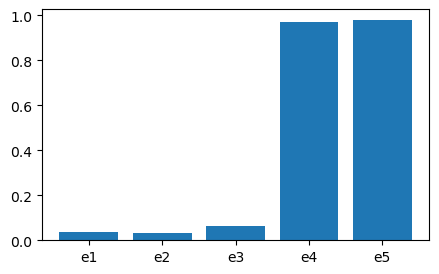
Results: {‘e1’: 0.036, ‘e2’: 0.031, ‘e3’: 0.059, ‘e4’: 0.928, ‘e5’: 0.934}
Component importance visualisation:
The BRC algorithm calculates system failure probability for general coherent systems.
It identifies (sub-)minimal survival and failure rules.
Identified rules are used to decompose system event space into failure and survival branches.
Branches can be used to compute advanced probability queries such as component importance measures.