Composite States and the C Matrix

The Problem: Exponential Explosion

Imagine you have a system with 20 binary components. A standard probability table — like a Bayesian network CPT — needs one row for every possible combination of states. That’s \(2^{20} = 1{,}048{,}576\) rows, and every new component doubles the table again.

This is where composite states come in. They’re the core idea behind the matrix-based Bayesian network (MBN) framework, and they let you collapse that million-row table into something manageable — often just a handful of rows.

Reference: Byun, J.-E. and Song, J. (2021). Generalized matrix-based Bayesian network for multi-state systems. Reliability Engineering & System Safety, 211, 107468. https://doi.org/10.1016/j.ress.2021.107468

What Is a Composite State?

A variable \(X\) with \(K\) states (indexed \(0, 1, \ldots, K{-}1\)) gets additional composite states — each one representing a subset of the original states bundled together.

MBNpy assigns these automatically via the B matrix. Here’s what it looks like for a three-state variable:

from mbnpy import variable

v = variable.Variable(name='x', values=[0, 1, 2])
print(v)

<Variable representing x['0', '1', '2'] at 0x1fd93373770>
+---------+-----------+
|   index | B         |
+=========+===========+
|       0 | {0}       |
+---------+-----------+
|       1 | {1}       |
+---------+-----------+
|       2 | {2}       |
+---------+-----------+
|       3 | {0, 1}    |
+---------+-----------+
|       4 | {0, 2}    |
+---------+-----------+
|       5 | {1, 2}    |
+---------+-----------+
|       6 | {0, 1, 2} |
+---------+-----------+

Index 3 means “state 0 or state 1.” Index 6 means “any state at all.” The power of this is that a single row in a probability table can now stand in for many exact-state combinations at once.

The C Matrix

The C matrix is the data structure at the heart of a CPM (Conditional Probability Matrix). Each row assigns a (possibly composite) state to every variable in the distribution, and a companion probability vector \(p\) gives each row’s probability.

A Concrete Example: Series System

Consider a series system \(S\) with four components \(X_1, X_2, X_3, X_4\). Each component is binary: 0 = failed, 1 = survived. The system fails if any component fails.

The brute-force table

Without composite states, you need all \(2^4 = 16\) combinations (columns: \([S,\; X_1,\; X_2,\; X_3,\; X_4]\)):

 S  X1  X2  X3  X4
[0   0   0   0   0]   <- system fails
[0   0   0   0   1]
[0   0   0   1   0]
[0   0   0   1   1]
[0   0   1   0   0]
[0   0   1   0   1]
[0   0   1   1   0]
[0   0   1   1   1]
[0   1   0   0   0]
[0   1   0   0   1]
[0   1   0   1   0]
[0   1   0   1   1]
[0   1   1   0   0]
[0   1   1   0   1]
[0   1   1   1   0]
[1   1   1   1   1]   <- system survives (all Xi = 1)

Since this is a deterministic function, every row has probability 1.

The compressed C matrix (5 rows instead of 16)

A series system has four minimal failure rules (one per component) and one survival rule. Using composite states, these map to just 5 rows:

 S  X1  X2  X3  X4
[0   0   2   2   2]   <- X1 fails; X2, X3, X4 can be anything  (8 combinations)
[0   1   0   2   2]   <- X1 survives, X2 fails; X3, X4 anything (4 combinations)
[0   1   1   0   2]   <- X1, X2 survive, X3 fails; X4 anything  (2 combinations)
[0   1   1   1   0]   <- X1, X2, X3 survive, X4 fails           (1 combination)
[1   1   1   1   1]   <- all survive                             (1 combination)

Here, composite state 2 means {0, 1} — “either failed or survived,” i.e. any state. The five rows cover all 16 combinations (\(8 + 4 + 2 + 1 + 1 = 16\)), and the probability vector is again all ones.

The compression ratio improves dramatically with scale: for \(N\) binary components, \(2^N\) rows collapse to just \(N + 1\). A system with a million components? That’s \(1{,}000{,}001\) rows instead of a number with over 300,000 digits.

The Overlap Trap

You might be tempted to write the C matrix like this — one row per component failure:

 S  X1  X2  X3  X4
[0   0   2   2   2]   <- fails if X1 = 0
[0   2   0   2   2]   <- fails if X2 = 0
[0   2   2   0   2]   <- fails if X3 = 0
[0   2   2   2   0]   <- fails if X4 = 0
[1   1   1   1   1]   <- survives

This looks clean, but it’s wrong. The rows overlap: the combination \((S{=}0,\; X_1{=}0,\; X_2{=}0,\; X_3{=}1,\; X_4{=}1)\) is counted by both the first row and the second. This double-counting inflates probabilities beyond 1 during inference.

The fix: branch and bound

The correct 5-row encoding avoids overlap by structuring the rows as a branch-and-bound decomposition — essentially a decision tree. The figure below shows this for the series system:

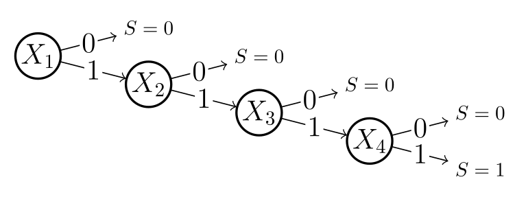
Branch-and-bound decomposition of the series system

Each branch in the tree corresponds directly to a row in the compressed C matrix:

\(X_1 \xrightarrow{0} S = 0\) — The leftmost branch: \(X_1\) fails, so the system fails regardless of the remaining components. Because \(X_2, X_3, X_4\) are never examined on this branch, they get composite state 2 (any state) → Row 1: [0 0 2 2 2], covering 8 combinations.
\(X_1 \xrightarrow{1} X_2 \xrightarrow{0} S = 0\) — \(X_1\) survives, but \(X_2\) fails. \(X_3\) and \(X_4\) are unexamined → Row 2: [0 1 0 2 2], covering 4 combinations.
\(X_1 \xrightarrow{1} X_2 \xrightarrow{1} X_3 \xrightarrow{0} S = 0\) — \(X_1\) and \(X_2\) survive, \(X_3\) fails. \(X_4\) is unexamined → Row 3: [0 1 1 0 2], covering 2 combinations.
\(X_1 \xrightarrow{1} X_2 \xrightarrow{1} X_3 \xrightarrow{1} X_4 \xrightarrow{0} S = 0\) — The first three survive, \(X_4\) fails → Row 4: [0 1 1 1 0], covering 1 combination.
\(X_1 \xrightarrow{1} X_2 \xrightarrow{1} X_3 \xrightarrow{1} X_4 \xrightarrow{1} S = 1\) — All survive → Row 5: [1 1 1 1 1], covering 1 combination.

Notice the pattern: variables that appear after the terminating branch are never reached, so they take the composite “any state” value. This is exactly why composite states enable compression — they encode “don’t care” conditions that arise naturally from the tree structure.

Because each path through the tree is mutually exclusive, no state combination is ever counted twice.

Key Takeaways

Composite states let a single C matrix row represent an entire family of state combinations. This transforms exponential-sized probability tables into compact, tractable representations — making it possible to run Bayesian inference on systems with thousands or millions of components.

The critical rule when building a C matrix: rows must never overlap. Branch-and-bound decomposition is a reliable way to guarantee this.