What and why mbnpy?

Tags: mbnpy

Last updated: 11 Aug 2024

More information about MBNPy can be found at MBNpy blog.

Motivation

Bayesian network (BN)

Bayesian network (BN) is a probabilistic graphical model (PGM). It visualises dependence between many random variables, which makes it much easier to formulate a high-dimensional probabilistic model.
In a BN graph, random variables are represented by circular nodes, and their dependence is represented by directed arrows.
_{*For more information about PGM, I strongly recommend Koller (2009).}

For example, let us consider an example BN in Fig. 1, which represents a system event subjected to some hazard risk. In the graph, random variables \(H\), \(X_1, \cdots, X_N\), and \(S\) respectively represent intensity of a hazard event, component events, and a system event.

In this problem, we can use BN to model causal relationship between the random variables. In Fig. 1, hazard \(H\) affects performance of components \(X_1,\cdots,X_N\), which then determine performance of system \(S\).

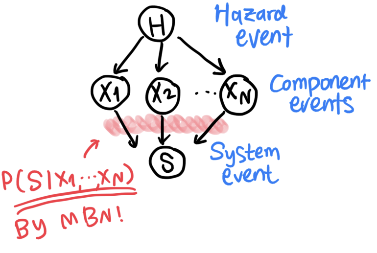
Once a BN graph is set up, each node is assigned a conditional probability on their parent nodes. For instance, the BN in Fig. 1 has $P(H)$, \(P(X_1 \left. \right\vert H),\cdots,P(X_N \left. \right\vert H)\), and \(P(S \left. \right\vert X_1, \cdots, X_N)\).

Then, the joint probability represented by the BN is simply the product of all these variables, i.e. \(P(S,X_1, \cdots, X_N,H)=P(S \left. \right\vert X_1, \cdots, X_N)\cdot P(X_1 \left. \right\vert H)\cdot \cdots \cdot P(X_N \left. \right\vert H)\cdot P(H).\)

Challenge: unaffordable memory

The challenge arises from the converging structure between \(X_1, \cdots, X_N\) and \(S\). Such structure naturally happens because a system’s state by definition depends on components’ states.

The challnege is that one needs to quantify the probability distribution \(P(S \left. \right\vert X_1,\cdots,X_N)\), whose dimension is as high as \((N+1)\).

If we have 30 component events and a system event, each having a binary state, we end up having to store \(2^{31}\approx 10^{9.3}\) probabilities to store, which is simply an impossible number.

Opportunity: Regularity in system events

There is a hope though: Many system functions are deterministic and show clear patterns, which can be encoded using much less memory than the actual number of existing instances.

For example, consider the reliability block diagram (RBD) in Fig. 2 (ref: Byun et al. 2019). The system consists of 8 component events, represented by random variables \(X_1,\cdots,X_8\). Each \(X_n\), \(n=1,\cdots,8\), takes a binary state of 0 (failure) and 1 (survival). Then, random variable \(S\) takes state 1 (survival) if vertex \(s\) and vertex \(t\) are connected and state 0, otherwise.

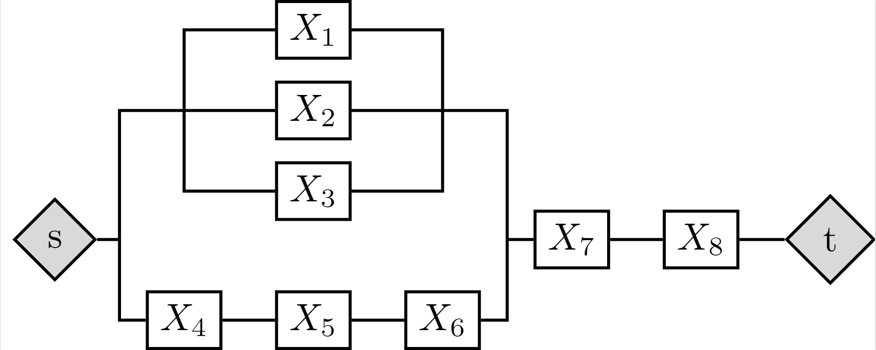
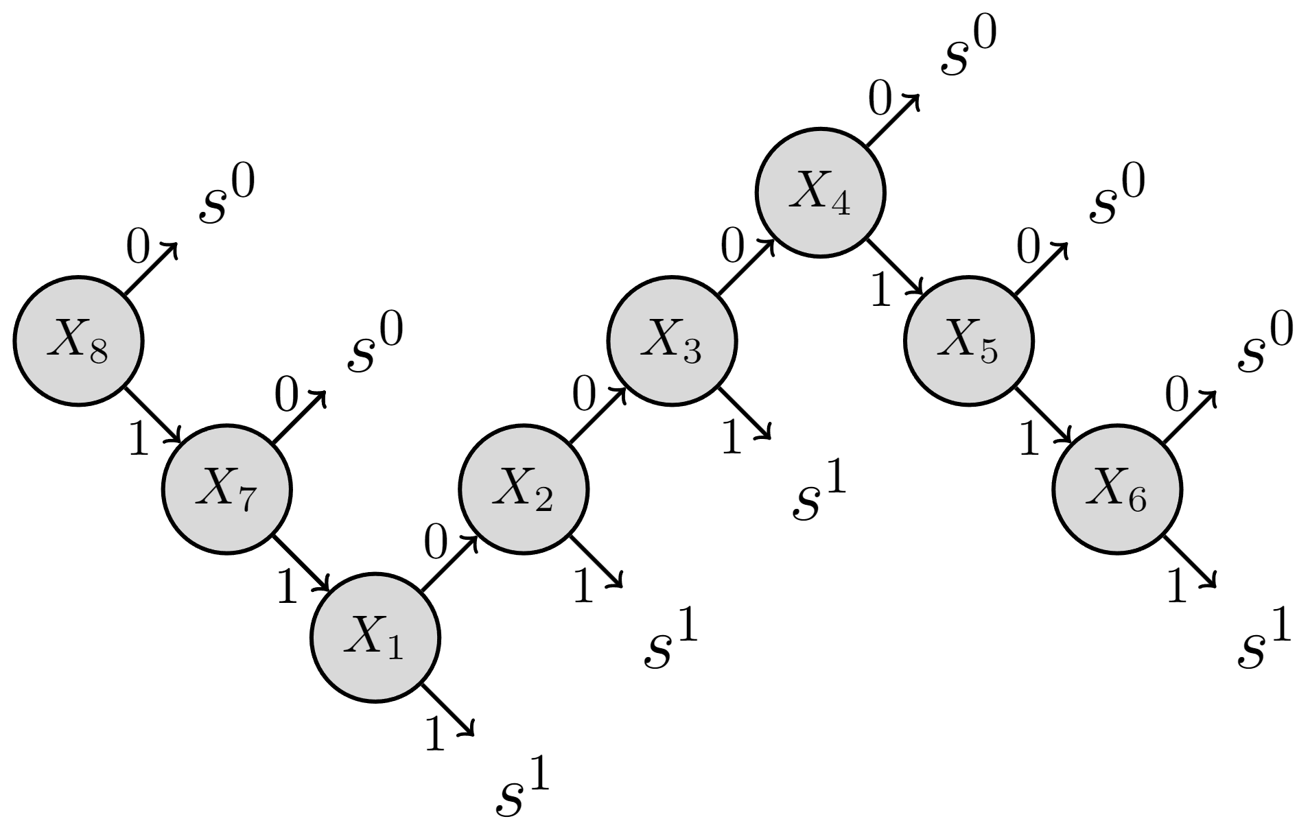
This means that there are \(2^{(8+1)}=512\) instances in total over \(X_1, \cdots, X_N, S\). However, if one applies branch and bound to decompose the event space, one can describe the whole event space by 9 branches as illustrated in Fig. 3 (ref: Byun et al. 2019).

For example, the leftmost branch at the top refers to that given \(X_8 = 0\) (abbreviated as \(x_8^0\)), the system fails (i.e. \(s^0\)). In other words, \(P(s^0 \left. \right\vert x_8^0) = 1\) and \(P(s^1 \left. \right\vert x_8^0) = 0\), regardless of other components’ states. Note that this single branch alone represents \(2^7=128\) instances (over \(X_1,\cdots,X_7\)).

Solution: Matrix-based Bayesian network (MBN)

MBN has been proposed as an alternative data structure of BN to handle large-scale systems (ref: Byun et al. 2019; Byun and Song 2021). It provides a means to encode patterns in \(P(S \left. \right\vert X_1,\cdots,X_N)\).

In the following demonstration, I will show how MBN can be used for encoding the branch and bound result in Fig 3. Detailed illustrations of this problem are available in Byun et al. (2019).

Demonstration: reliability block diagram (RBD)

Referring to Figs 1-3, I will show how we can quantify probability distributions using mbnpy toolkit.

mbnpy toolkit

For the following calculations, we use mbnpy toolkit available at GitHub. Below, we are assuming that conda environment bns has been activated already–this can be done by using the file BNS_JT_py3.9.yml.

Now, we import mbnpy toolkit.

from BNS_JT import cpm, variable
import numpy as np

Quantification of probability distributions

mbnpy requires two data structures: Conditional Probability Matrices (CPMs) and Variables. CPMs store probability distributions, and variables store information of each variable in a BN.

We first create those two data structures as a dictionary (a Python’s data structure).

cpms = {} 
varis = {} 

(1) Hazard node

Random variable \(H\) represents insensity of a hazard event. It has 3 states, 0 (mild), 1 (moderate), and 2 (intense).

The probability distribution is given as \(P(h^0)=0.6, P(h^1)=0.3, P(h^2)=0.1.\)

varis['haz'] = variable.Variable(name = 'haz', B=np.eye(3), values=['mild', 'moderate', 'intensity'] )
cpms['haz'] = cpm.Cpm( variables=[varis['haz']], no_child=1, C=np.array([0, 1, 2]), p = [0.6, 0.3, 0.1] )

There are a few things to note here about using mbnpy.

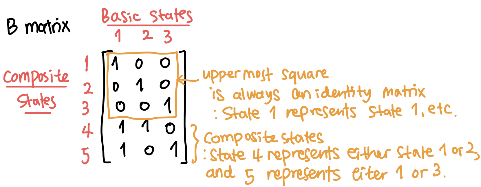
First, in a B matrix, which is introduced by Byun and Song (2021), each row represents a state (both basic and composite state), and each column represents a basic state, only.

For example, consider a B matrix in Fig 4. There are three basic states as there are three columns, and five states in total being represented by the five rows.

In each row, the basic state(s) represented by a state has its column value as 1 and otherwise, 0. By construction, the uppermost part is always an identity matrix, and following rows represent a composite state. In Fig 4, the composite state 4 represents either 1 or 2, and state 5 either 1 or 3.

The necessity of composite states will become clearer when handling the system event.

Second, Variable takes its third input as values, which should be a list having the same length as the number of basic states. It is to record what each state means, simply for convenience.

Third, a Cpm’s first input is a list of variables in its scope and second variable as the number of child variables among them. Note that the toolkit assumes that the first no_child variables in variables are considered child nodes and the rest are parent (or conditional) nodes.

Fourth, the third and the fourth inputs of Cpm are respectively states and probabilities of each instance. The same row of C and p must indicates the same instance.

(2) Component events

The component event \(X_n\), \(n=1,\cdots,8\), takes a binary state, 0 (failure) and 1 (survival). The probability distributions are set as \(P(x^0|h^0)=0.05, P(x^1|h^0)=0.95, P(x^0|h^1)=0.10\), \(P(x^1|h^1)=0.90, P(x^0|h^2)=0.20, P(x^1|h^2)=0.80\),
for \(n=1,2,3\), and
\(P(x^0|h^0)=0.01, P(x^1|h^0)=0.99, P(x^0|h^1)=0.05\), \(P(x^1|h^1)=0.95, P(x^0|h^2)=0.10, P(x^1|h^2)=0.90\),
for \(n=4,5,6,7,8\).

This can be coded as below. It is noted that now we introduce a composite state 2 that represents either 0 or 1 using the B matrix.

no_comp = 8

for n in range(3):
    x_name = 'x'+str(n+1)
    varis[x_name] = variable.Variable(
                        name = x_name,
                        B=np.vstack([np.eye(2), [1, 1]]),
                        values=['fail', 'survive'] )
    cpms[x_name] = cpm.Cpm(
                        variables=[varis[x_name], varis['haz']],
                        no_child=1,
                        C=np.array([[0, 0], [1, 0], [0, 1],
                                    [1,1], [0,2], [1,2]]),
                        p = [0.05,0.95,0.10,
                            0.90,0.20,0.80] )

for n in range(3,8):
    x_name = 'x'+str(n+1)
    varis[x_name] = variable.Variable(
                        name = x_name
                        B=np.vstack([np.eye(2), [1, 1]]),
                        values=['fail', 'survive'] )
    cpms[x_name] = cpm.Cpm(
                        variables=[varis[x_name], varis['haz']],
                        no_child=1,
                        C=np.array([[0, 0], [1, 0], [0, 1],
                                    [1,1], [0,2], [1,2]]),
                        p = [0.01,0.99,0.05,
                            0.95,0.10,0.90] )

If one prints out the CPMs of \(X_1\) and \(X_4\),

print( cpms['x1'] )
print( cpms['x4'] )

one gets

Cpm(variables=['x1', 'haz'], no_child=1, C=[[0 0]
    [1 0]
    [0 1]
    [1 1]
    [0 2]
    [1 2]], p=[[0.05]
    [0.95]
    [0.1 ]
    [0.9 ]
    [0.2 ]
    [0.8 ]]
Cpm(variables=['x4', 'haz'], no_child=1, C=[[0 0]
    [1 0]
    [0 1]
    [1 1]
    [0 2]
    [1 2]], p=[[0.01]
    [0.99]
    [0.05]
    [0.95]
    [0.1 ]
    [0.9 ]]

(3) System event

To encode the system event’s distribution, the branch and bound result in Fig 3 is used as below. Note that this is where \(x_n^2\) (\(:=(X_n=2)\)) comes into the play.

varis['sys'] = variable.Variable(
                        name='sys',
                        B=np.eye(2),
                        values=['fail', 'survive'] )

Cs = np.array([[0, 2, 2, 2, 2, 2, 2, 2, 0],
               [0, 2, 2, 2, 2, 2, 2, 0, 1],
               [1, 1, 2, 2, 2, 2, 2, 1, 1],
               [1, 0, 1, 2, 2, 2, 2, 1, 1],
               [1, 0, 0, 1, 2, 2, 2, 1, 1],
               [0, 0, 0, 0, 0, 2, 2, 1, 1],
               [0, 0, 0, 0, 1, 0, 2, 1, 1],
               [0, 0, 0, 0, 1, 1, 0, 1, 1],
               [1, 0, 0, 0, 1, 1, 1, 1, 1]])
ps = np.array( [1,1,1,1,1,1,1,1,1] )

cpms['sys'] = cpm.Cpm(
                variables=[varis['sys']]+
                    [varis['x'+str(n+1)] for n in range(no_comp)],
                no_child=1,
                C=Cs,
                p=ps)

When one prints out

print(cpms['sys'])

it shows

Cpm(variables=['sys', 'x1', 'x2', 'x3', 'x4', 'x5', 'x6', 'x7', 'x8'], no_child=1, C=[[0 2 2 2 2 2 2 2 0]
    [0 2 2 2 2 2 2 0 1]
    [1 1 2 2 2 2 2 1 1]
    [1 0 1 2 2 2 2 1 1]
    [1 0 0 1 2 2 2 1 1]
    [0 0 0 0 0 2 2 1 1]
    [0 0 0 0 1 0 2 1 1]
    [0 0 0 0 1 1 0 1 1]
    [1 0 0 0 1 1 1 1 1]], p=[[1]
    [1]
    [1]
    [1]
    [1]
    [1]
    [1]
    [1]
    [1]]

In the CPM (represented by Cs and ps), each row represents each branch in Fig 3 from left to right. For example, the first row means that the system fails–\(s^0\), given \(X_8\)’s failure–\(x_8^0\), and all other component states do not matter– \(x_n^2\) for \(n=1,\cdots,7\).

Using CPM, the 512 instances can be represented by \(9 \cdot (1+8) + 9 \cdot 1=90\) elements (i.e. (elements in Cs)+(elements in ps)). The reduction in memory becomes more dramatic as the number of component events increases.

In the code above, there are two noteworthy points about quantifying a CPM:

1. The instances represented by each row must be mutually exclusive so that they will not be double counted during the inference.
2. Instances with zero probability are excluded from a CPM because they have no effects on inference results. For example, the counterpart instance of the first row has zero probability, i.e. \(P(s^1 \left. \right\vert x_8^0)=0\), so it is not included in the CPM.

Next step: Inference

We can now use inference operations (i.e. conditioning, product, and sum) to calculate a system failure probability, i.e. (in the example above) the probability of node \(s\) and \(t\) being disconnected given an occurrence of a hazard event.

This can be done using mbnpy as well. Performing an inferece will be posted in another article.

References

Byun, J. E. & Song, J. (2021). Generalized matrix-based Bayesian network for multi-state systems. Reliability Engineering & System Safety, 211, 107468.
Byun, J. E., Zwirglmaier, K., Straub, D. & Song, J. (2019). Matrix-based Bayesian Network for efficient memory storage and flexible inference. Reliability Engineering & System Safety, 185, 533-545.
Koller, D. & Friedman, N. (2009). Probabilistic graphical models: principles and techniques. MIT press.