EMA aftershock example

This example builds a Bayesian network for earthquake mainshock-aftershock analysis on the Eastern Massachusetts highway network. It combines regional seismicity, edge-level ground motion and damage, binary component survival, and a system-state classifier based on RSR reference sets.

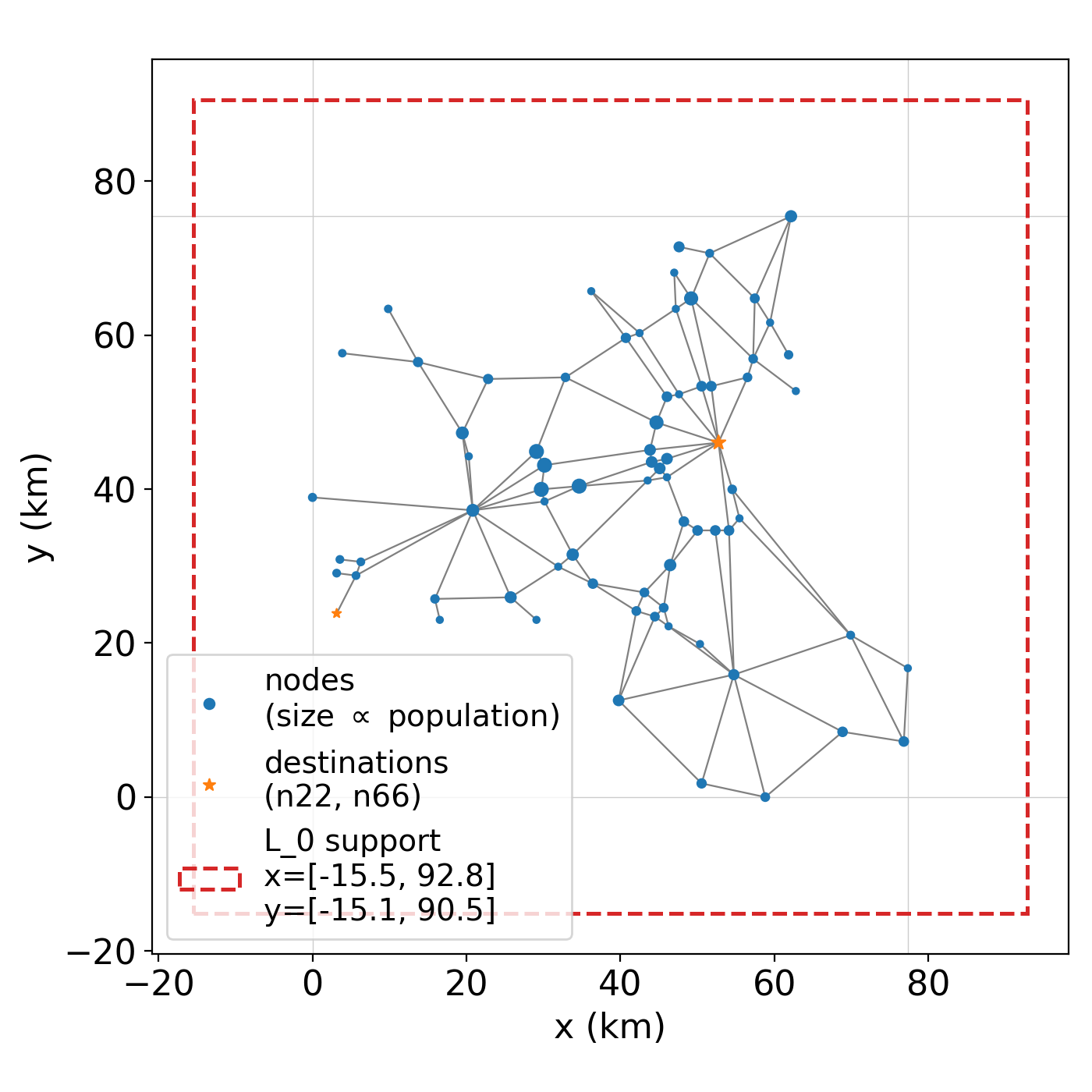
The full mathematical model is described in EMA_aftershock_models.pdf. The EMA benchmark network and the hypothetical areal seismic source zone are shown below:

The main BN structure is:

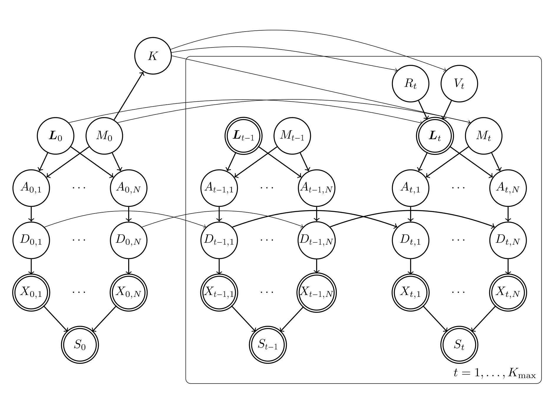
At a high level, the model has one mainshock and up to K_max aftershock slots. The mainshock has location L_0, magnitude M_0, and induced edge variables A_{0,n}, D_{0,n}, and X_{0,n}. The number of aftershocks K is sampled from M_0. Each aftershock slot t has distance R_t, angle V_t, location L_t, magnitude M_t, and the same edge-level sequence A_{t,n}, D_{t,n}, and X_{t,n}. The system state S_t is computed from all component states X_{t,n}.

The example workflow has three analysis steps:

1. Define the BN variables and probability objects.

2. Run unconditional forward sampling and summarise prior behaviour.

3. Estimate P(S_t | X_{0,n}=0) by modifying a damage node P(D_{0,n} | A_{0,n}).

Step 1: define the model

The file examples/EMA_aftershock/s01_define_model.py assembles the BN. It provides helper functions to load the highway topology, load RSR reference sets, create variables, and attach each variable to its probability object.

The main inputs are:

• data/nodes.json and data/edges.json for the EMA highway topology.

• data/probs_eq.json for edge-level single-shock survival/failure data.

• rsr_res/refs_up_*.pt and rsr_res/refs_low_*.pt for system-state classification.

The key construction functions are:

• load_topology() reads nodes and edges and computes edge midpoints.

• load_rsr_refs() loads the reference tensors used by S_t.

• define_variables() creates names such as L_x_0, M_0, K, A_0_e0001, D_0_e0001, X_0_e0001, and S_0.

• define_probs() creates the corresponding probability objects from l.py, m.py, k.py, r.py, v.py, a.py, d.py, x.py, and s.py.

The model separates L_x and L_y into different variables because the inference engine expects each probability object to own a unique child variable name. Mainshock location coordinates are independent uniforms, while aftershock coordinates are deterministic functions of L_0, R_t, and V_t.

"""
Assemble the BN for the EMA mainshock-aftershock example.

The model includes:

* Mainshock variables — L_0 (split into L_x_0, L_y_0), M_0, K and, for
  each edge n: A_{0,n}, D_{0,n}, X_{0,n}. The system state S_0.
* Aftershock slots ``t = 1, ..., K_max`` — R_t, V_t, L_x_t, L_y_t, M_t,
  and per-edge A_{t,n}, D_{t,n}, X_{t,n}, plus S_t.

For tractability you can pass smaller ``K_max`` / ``edge_subset`` values;
the default reads the full EMA topology from ``./data/``.
"""

import json
import os
import sys
from pathlib import Path

import numpy as np
import torch

BASE = Path(__file__).resolve().parent
sys.path.insert(0, str(BASE))

REPO_ROOT = BASE.parent.parent
if str(REPO_ROOT) not in sys.path:
    sys.path.insert(0, str(REPO_ROOT))

# Optional: add rsr repo if it lives next to tbnpy
RSR_REPO = REPO_ROOT.parent / "rsr"
if RSR_REPO.exists() and str(RSR_REPO) not in sys.path:
    sys.path.insert(0, str(RSR_REPO))

from tbnpy import variable

try:
    from ndtools import fun_binary_graph as fbg  # type: ignore[import]
    from ndtools.graphs import build_graph        # type: ignore[import]
except ImportError:
    fbg = None
    build_graph = None

import l as l_mod
import m as m_mod
import k as k_mod
import r as r_mod
import v as v_mod
import a as a_mod
import d as d_mod
import x as x_mod
import s as s_mod


DATA_DIR = BASE / "data"
RSR_DIR = BASE / "rsr_res"


def load_topology(edge_subset=None):
    """Load EMA nodes/edges and compute each edge's midpoint (x, y)."""
    with open(DATA_DIR / "nodes.json", "r") as f:
        nodes = json.load(f)
    with open(DATA_DIR / "edges.json", "r") as f:
        edges = json.load(f)

    if edge_subset is not None:
        keep = set(edge_subset)
        edges = {k: v for k, v in edges.items() if k in keep}

    midpoints = {}
    for e_id, e in edges.items():
        a = nodes[e["from"]]
        b = nodes[e["to"]]
        midpoints[e_id] = ((a["x"] + b["x"]) / 2.0, (a["y"] + b["y"]) / 2.0)

    return nodes, edges, midpoints


def load_rsr_refs(max_st=2, device="cpu"):
    """Load the upper/lower reference tensors built for the EMA system."""
    refs_upper, refs_lower = {}, {}
    for s_st in range(1, max_st + 1):
        refs_upper[s_st] = torch.load(
            RSR_DIR / f"refs_up_{s_st}.pt", map_location=device
        )
        refs_lower[s_st] = torch.load(
            RSR_DIR / f"refs_low_{s_st - 1}.pt", map_location=device
        )
    return refs_upper, refs_lower


def make_s_fun(dests=None):
    """Build and return an ``s_fun`` callable for use with :class:`s_mod.S`.

    Uses ``fbg.eval_population_accessibility`` (ndtools) to resolve component
    states that the RSR classifier leaves unknown.
    """
    assert fbg is not None and build_graph is not None, (
        "ndtools is not importable; make sure the ndtools repo is on sys.path"
    )
    if dests is None:
        dests = ["n22", "n66"]

    with open(DATA_DIR / "nodes.json") as f:
        nodes = json.load(f)
    with open(DATA_DIR / "edges.json") as f:
        edges = json.load(f)
    with open(DATA_DIR / "probs_eq.json") as f:
        probs_dict = json.load(f)

    G_base = build_graph(nodes, edges, probs_dict)

    def s_fun(comps_st):
        conn_pop_ratio, sys_st, _ = fbg.eval_population_accessibility(
            comps_st, G_base, dests,
            avg_speed=60.0,
            target_time_max=0.25,
            target_pop_max=[0.95, 0.99],
            length_attr="length_km",
            population_attr="population",
        )
        return conn_pop_ratio, sys_st, None

    return s_fun


def region_from_nodes(nodes, margin_frac=0.20):
    """Bounding box of node coordinates, expanded by ``margin_frac`` on each side.

    ``margin_frac`` is relative to the span of the data in that axis, so a
    value of 0.20 adds 20% of the x-range on the left and right, and 20%
    of the y-range at the top and bottom.
    """
    xs = [n["x"] for n in nodes.values()]
    ys = [n["y"] for n in nodes.values()]
    x_min, x_max = min(xs), max(xs)
    y_min, y_max = min(ys), max(ys)
    dx = (x_max - x_min) * margin_frac
    dy = (y_max - y_min) * margin_frac
    return (x_min - dx, x_max + dx, y_min - dy, y_max + dy)


def define_variables(edge_names, K_max=3, max_st=2):
    """Create all tbnpy Variable instances.

    System-state variables ``S_i`` take values ``{0, 1, ..., max_st}`` —
    states are 0-indexed, matching the RSR ref-dict convention where
    ``refs_up_{s}`` / ``refs_low_{s-1}`` describe the boundary between
    ``S >= s`` and ``S <= s - 1``.
    """
    varis = {}
    cont = lambda name: variable.Variable(name=name, values=(-torch.inf, torch.inf))

    sys_states = list(range(max_st + 1))  # 0..max_st

    # Mainshock
    varis["L_x_0"] = cont("L_x_0")
    varis["L_y_0"] = cont("L_y_0")
    varis["M_0"] = cont("M_0")
    varis["K"] = variable.Variable(name="K", values=list(range(K_max + 1)))

    for n in edge_names:
        varis[f"A_0_{n}"] = cont(f"A_0_{n}")
        varis[f"D_0_{n}"] = cont(f"D_0_{n}")
        varis[f"X_0_{n}"] = variable.Variable(name=f"X_0_{n}", values=[0, 1])
    varis["S_0"] = variable.Variable(name="S_0", values=sys_states)

    # Aftershock slots
    for t in range(1, K_max + 1):
        varis[f"R_{t}"] = cont(f"R_{t}")
        varis[f"V_{t}"] = cont(f"V_{t}")
        varis[f"L_x_{t}"] = cont(f"L_x_{t}")
        varis[f"L_y_{t}"] = cont(f"L_y_{t}")
        varis[f"M_{t}"] = cont(f"M_{t}")
        for n in edge_names:
            varis[f"A_{t}_{n}"] = cont(f"A_{t}_{n}")
            varis[f"D_{t}_{n}"] = cont(f"D_{t}_{n}")
            varis[f"X_{t}_{n}"] = variable.Variable(
                name=f"X_{t}_{n}", values=[0, 1]
            )
        varis[f"S_{t}"] = variable.Variable(name=f"S_{t}", values=sys_states)

    return varis


def define_probs(varis, edges, midpoints, region,
                 refs_upper, refs_lower, K_max=3,
                 s_fun=None, device="cpu"):
    """Create all probability objects keyed by their child variable name."""
    edge_names = list(edges.keys())
    probs = {}

    # ---- Mainshock ----
    x_min, x_max, y_min, y_max = region
    probs["L_x_0"] = l_mod.L0(
        childs=[varis["L_x_0"]], low=x_min, high=x_max, device=device,
    )
    probs["L_y_0"] = l_mod.L0(
        childs=[varis["L_y_0"]], low=y_min, high=y_max, device=device,
    )
    probs["M_0"] = m_mod.M0(childs=[varis["M_0"]], device=device)
    probs["K"] = k_mod.K(
        childs=[varis["K"]], parents=[varis["M_0"]],
        K_max=K_max, device=device,
    )

    for n in edge_names:
        probs[f"A_0_{n}"] = a_mod.A(
            childs=[varis[f"A_0_{n}"]],
            parents=[varis["M_0"], varis["L_x_0"], varis["L_y_0"]],
            edge_midpoint=midpoints[n], device=device,
        )
        probs[f"D_0_{n}"] = d_mod.D0(
            childs=[varis[f"D_0_{n}"]],
            parents=[varis[f"A_0_{n}"]], device=device,
        )
        probs[f"X_0_{n}"] = x_mod.X(
            childs=[varis[f"X_0_{n}"]],
            parents=[varis[f"D_0_{n}"]], device=device,
        )

    probs["S_0"] = s_mod.S(
        childs=[varis["S_0"]],
        parents=[varis[f"X_0_{n}"] for n in edge_names],
        refs_dict_upper=refs_upper, refs_dict_lower=refs_lower,
        row_names=edge_names, s_fun=s_fun, device=device,
    )

    # ---- Aftershocks ----
    for t in range(1, K_max + 1):
        probs[f"R_{t}"] = r_mod.R(
            childs=[varis[f"R_{t}"]], parents=[varis["K"]],
            slot_idx=t, device=device,
        )
        probs[f"V_{t}"] = v_mod.V(
            childs=[varis[f"V_{t}"]], parents=[varis["K"]],
            slot_idx=t, device=device,
        )
        probs[f"L_x_{t}"] = l_mod.Lt(
            childs=[varis[f"L_x_{t}"]],
            parents=[varis["L_x_0"], varis[f"R_{t}"], varis[f"V_{t}"]],
            axis="x", device=device,
        )
        probs[f"L_y_{t}"] = l_mod.Lt(
            childs=[varis[f"L_y_{t}"]],
            parents=[varis["L_y_0"], varis[f"R_{t}"], varis[f"V_{t}"]],
            axis="y", device=device,
        )
        probs[f"M_{t}"] = m_mod.Mt(
            childs=[varis[f"M_{t}"]],
            parents=[varis["M_0"], varis["K"]],
            slot_idx=t, device=device,
        )

        for n in edge_names:
            probs[f"A_{t}_{n}"] = a_mod.A(
                childs=[varis[f"A_{t}_{n}"]],
                parents=[varis[f"M_{t}"], varis[f"L_x_{t}"], varis[f"L_y_{t}"]],
                edge_midpoint=midpoints[n], device=device,
            )
            probs[f"D_{t}_{n}"] = d_mod.Dt(
                childs=[varis[f"D_{t}_{n}"]],
                parents=[varis[f"A_{t}_{n}"], varis[f"D_{t - 1}_{n}"]],
                device=device,
            )
            probs[f"X_{t}_{n}"] = x_mod.X(
                childs=[varis[f"X_{t}_{n}"]],
                parents=[varis[f"D_{t}_{n}"]], device=device,
            )

        probs[f"S_{t}"] = s_mod.S(
            childs=[varis[f"S_{t}"]],
            parents=[varis[f"X_{t}_{n}"] for n in edge_names],
            refs_dict_upper=refs_upper, refs_dict_lower=refs_lower,
            row_names=edge_names, s_fun=s_fun, device=device,
        )

    return probs


if __name__ == "__main__":
    device = "cuda" if os.environ.get("USE_CUDA", "0") == "1" else "cpu"
    K_max = 2     # keep small for the smoke test
    max_st = 2    # S in {0, 1, 2}; matches the rsr_res files

    nodes, edges, midpoints = load_topology()
    region = region_from_nodes(nodes)
    refs_upper, refs_lower = load_rsr_refs(max_st=max_st, device=device)

    varis = define_variables(list(edges.keys()), K_max=K_max, max_st=max_st)
    probs = define_probs(varis, edges, midpoints, region,
                         refs_upper, refs_lower, K_max=K_max, device=device)

    print(f"Defined {len(varis)} variables and {len(probs)} probability nodes.")

Step 2: forward inference

The file examples/EMA_aftershock/s02_forward_inference.py performs prior forward inference with no evidence. It builds the full BN using s01_define_model.py and samples every variable:

filled = inference.sample(
    probs=probs,
    query_nodes=query_nodes,
    n_sample=n_sample,
    batch_size=50_000,
)

The batch_size argument controls how many samples are generated at once, so that a large number of samples can be generated without running out of memory.

The script writes two kinds of output:

• results/forward_stats_Kmax{K}_maxst{M}_n{N}.csv with long-form summary statistics.

• results/histograms/Kmax{K}_maxst{M}_n{N}/ with one histogram PNG per variable.

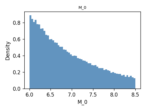
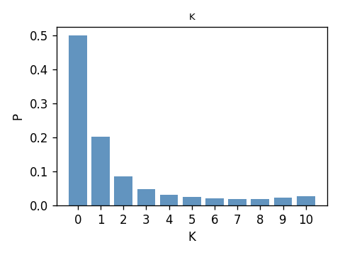
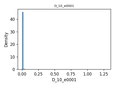
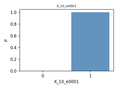
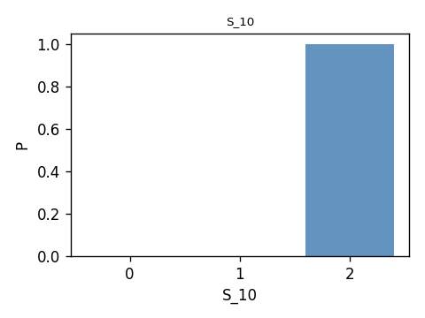
Representative prior histograms are shown below.

Run the script from the example directory:

cd examples/EMA_aftershock
python s02_forward_inference.py

Step 3: conditioning on component failure

The file examples/EMA_aftershock/s03_cal_s_x0.py estimates

\[P(S_t \mid X_{0,n}=0)\]

for each edge n and each time slice t. Here X_{0,n}=1 means that edge n survives the mainshock, so X_{0,n}=0 means the edge fails.

The conditioning is implemented by a small model surgery. Since X_{0,n} is a deterministic threshold of D_{0,n}, the script replaces the original probability object for D_{0,n} with DeltaD:

probs_mod[f"D_0_{edge_id}"] = DeltaD(
    childs=[varis[f"D_0_{edge_id}"]],
    parents=orig.parents,
    value=1.0,
    device=device,
)

This sets D_{0,n}=1.0 regardless of the values of its parent variables. Because 1.0 is above the damage threshold used by X_{0,n}, the modified BN represents the event X_{0,n}=0. Forward sampling under this modified model therefore gives Monte Carlo samples from P(S_t | X_{0,n}=0):

marg = estimate_S_marginals(
         probs_mod,
         varis,
         K_max,
         n_sample,
         max_st=max_st,
         batch_size=batch_size,
     )

where estimate_S_marginals() is a helper function that runs forward sampling using inference.sample with the updated probabilities probs_mod.

The surrogate node keeps the original parents so that ancestor ordering and downstream dependencies remain valid, but its sample and log_prob methods ignore those parent values.

The output is a long-form CSV:

results/S_given_X0_zero_Kmax{K}_maxst{M}_n{N}.csv

with columns:

• edge

• t

• S

• P(S_t=S | X_0_n=0)

• cov, the coefficient of variation of the empirical probability estimate

Run the script from the example directory:

cd examples/EMA_aftershock
python s03_cal_s_x0.py

The __main__ block can be adjusted for larger or smaller sample budgets, GPU use, and a subset of target edges.

Computational cost scaling

The file examples/EMA_aftershock/s04_eval_performance.py benchmarks how the wall-clock cost of forward sampling changes as the number of Monte Carlo samples increases. By default, it samples all variables in the EMA BN, matching the forward-sampling setup used in s02_forward_inference.py.

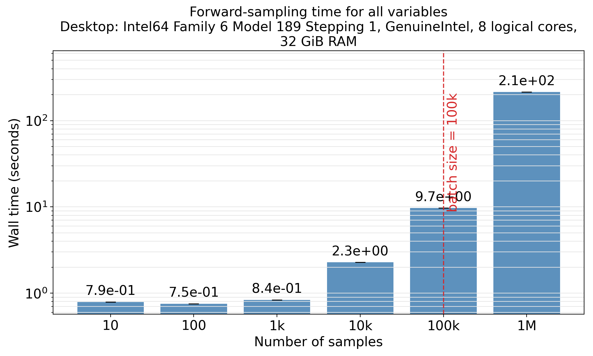
The cost generally increases with the number of samples, but the scaling benefit from vectorisation diminishes as the requested sample count reaches the internal batch_size. Beyond that point, the sampler splits the work into multiple batches, which adds overhead and can make the computation scale less smoothly.

Run the benchmark from the example directory:

cd examples/EMA_aftershock
python s04_eval_performance.py