ABCDE example

This example demonstrates how TBN performs inference on a Bayesian network that combines discrete and continuous variables, using tensorised Monte Carlo sampling and adaptive MCMC.

The example is intentionally minimal, but it exercises the full workflow: model definition, evidence conditioning, scalable inference, and posterior analysis.

Model structure

The Bayesian network consists of six variables:

• A: discrete, two states

• B: discrete, three states

• C: continuous, conditioned on (A, B)

• OC: continuous observation of C

• D: binary

• E: continuous, deterministic function of (C, D)

The BN graph is:

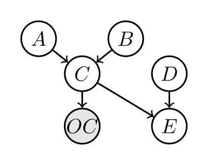
OC is shaded as an observed variable.

Task

Given multiple noisy observations of OC, the task is to infer the posterior distributions of A, B, and C, i.e. \(p(A, B, C \mid OC=\text{evidence})\).

Step 0: Define custom variables and probability distributions

A, B, and D are discrete, tractable (i.e. small state-space) variables, so they use built-in CPT classes.

C, OC, and E are continuous (or non-tabular) variables, requiring custom probability models:

• C | A, B: Gaussian distribution with mean and variance depending on the discrete parents (A, B):

  import torch
  from torch.distributions import Normal
  
  class C:
      def __init__(self, childs, parents, sigma=0.6, device="cpu"):
          """
          C | A,B ~ Normal(A + B, sigma^2)
  
          childs  : [Variable C]
          parents : [Variable A, Variable B]
          sigma   : fixed noise std (float)
          """
          self.childs = childs
          self.parents = parents
          self.device = device
  
          self.sigma = float(sigma)
  
          # parent variables
          self.A = parents[0]
          self.B = parents[1]
  
          # value lookup tables
          self.A_values = torch.tensor(
              self.A.values, dtype=torch.float32, device=device
          )
          self.B_values = torch.tensor(
              self.B.values, dtype=torch.float32, device=device
          )
  
      # ------------------------------------------------------------------
      def sample(self, Cs_pars):
          """
          Cs_pars : (N, 2)
              Cs_pars[:,0] = A index
              Cs_pars[:,1] = B index
  
          Returns
          -------
          Cs   : (N,) sampled C values
          logp : (N,) log p(C | A,B)
          """
          Cs_pars = Cs_pars.to(self.device).long()
  
          A_idx = Cs_pars[:, 0]
          B_idx = Cs_pars[:, 1]
  
          mean = self.A_values[A_idx] + self.B_values[B_idx]
          std = torch.full_like(mean, self.sigma)
  
          dist = Normal(mean, std)
          Cs = dist.sample()
          logp = dist.log_prob(Cs)
  
          return Cs, logp
  
      # ------------------------------------------------------------------
      def log_prob(self, Cs):
          """
          Cs : (N, 3)
              Cs[:,0] = C value
              Cs[:,1] = A index
              Cs[:,2] = B index
  
          Returns
          -------
          log p(C | A,B) : (N,)
          """
          Cs = Cs.to(self.device)
  
          C_val = Cs[:, 0]
          A_idx = Cs[:, 1].long()
          B_idx = Cs[:, 2].long()
  
          mean = self.A_values[A_idx] + self.B_values[B_idx]
          std = torch.full_like(mean, self.sigma)
  
          dist = Normal(mean, std)
          return dist.log_prob(C_val)
  

• OC | C: Noisy observation model with Gaussian noise:

  import torch
  from torch.distributions import Normal
  
  class OC:
      def __init__(self, childs, parents, device='cpu'):
          """
          childs: [OC variable]
          parents: [C variable]
          OC = C + Normal(0, 1)
          """
          self.childs = childs
          self.parents = parents
          self.device = device
  
          # standard deviation is fixed
          self.std = torch.tensor(0.5, device=device)
  
      # --------------------------------------------------------------
      def sample(self, Cs_pars):
          """
          Cs_pars: tensor (N, 1)
              Cs_pars[:,0] = C value
  
          Returns:
              OC samples of shape (N,)
          """
          Cs_pars = Cs_pars.to(self.device)
          C_val = Cs_pars[:, 0]
  
          dist = Normal(C_val, self.std)
          Cs = dist.rsample()  # (N,)
          ps = dist.log_prob(Cs)  # (N,)
  
          return Cs, ps  
  
      # --------------------------------------------------------------
      def log_prob(self, Cs):
          """
          Cs: tensor (N, 2)
              Cs[:,0] = observed OC value 
              Cs[:,1] = C value
  
          Returns:
              log p(OC | C), tensor shape (N,)
          """
          Cs = Cs.to(self.device)
  
          OC_val  = Cs[:, 0]
          C_val = Cs[:, 1]
  
          dist = Normal(C_val, self.std)
          return dist.log_prob(OC_val)   # (N,)
  

• E | C, D: Deterministic relation defined by a function:

  import torch
  
  class E:
      def __init__(self, childs, parents, device='cpu'):
          """
          childs: list [E] (unused but consistent with your structure)
          parents: list [C, D]
              C: continuous-valued parent (tensor-like values for samples)
              D: binary parent (0 or 1)
          """
          self.childs = childs
          self.parents = parents
          self.device = device
  
      # ------------------------------------------------------------------
      def sample(self, Cs_pars):
          """
          Cs_pars: (N, 2)
              Cs_pars[:,0] = C value   (float)
              Cs_pars[:,1] = D index   (0 or 1)
          
          Returns:
              E samples (N,)
          """
          Cs_pars = Cs_pars.to(self.device)
  
          C_val = Cs_pars[:, 0]
          D_idx = Cs_pars[:, 1].long()
  
          # E = C if D==0, else 0
          Cs = torch.where(D_idx == 0, C_val, torch.zeros_like(C_val))
  
          # deterministic function, i.e. P(E | C, D) = 1
          n_sample = Cs_pars.shape[0]
          ps = torch.log(torch.ones(n_sample,)).to(self.device)
  
          return Cs, ps
  
      # ------------------------------------------------------------------
      def log_prob(self, Es):
          """
          Es: shape (N, 3)
              Es[:,0] = E value
              Es[:,1] = C value 
              Es[:,2] = D state (0 or 1) 
          
          Returns:
              log p(E | C, D) of shape (N,)
          """
  
          Es = Es.to(self.device)
  
          E_val = Es[:, 0]
          C_val = Es[:, 1]
          D_idx = Es[:, 2].long()
  
          # Deterministic rule: valid_E = C if D==0 else 0
          expected_E = torch.where(D_idx == 0, C_val, torch.zeros_like(C_val))
  
          # Valid if E_val == expected_E
          is_valid = (E_val == expected_E)
  
          # log 1 = 0 for valid, log 0 = -inf for invalid
          logp = torch.where(is_valid, torch.zeros_like(E_val), torch.full_like(E_val, -float("inf")))
  
          return logp
  

Important notes

A custom probability model class should include (at minimum) the following methods:

1. __init__ defines core properties such as childs, parents, and device (cpu or gpu). Additional properties may be added as needed.

2. sample generates samples of child variables conditioned on given samples of the parent nodes.

   • Inputs: self and Cs_pars, where Cs_pars is a tensor of shape (num_samples, num_parents) storing realisations of the parent variables.

   • Returns: - (recommended) a tensor of child samples of shape (num_samples, num_childs) - a tensor of log-probabilities of shape (num_samples,) for the generated samples

3. log_prob computes the log-probability of given samples.

   • Inputs: self and Cs, where Cs is a tensor of shape (num_samples, num_childs + num_parents) storing realisations of both child (first) and parent (second) variables.

   • Returns: a tensor of shape (num_samples,) storing log-probabilities.

All methods should be compatible with both CPU and GPU tensors and should use PyTorch tensor operations for efficiency.

Step 1: defining variables and probability models

The file s1_define_model.py defines:

1. Variables (discrete vs. continuous)

2. Conditional probability objects for each node

In particular:

• P(A) and P(B) are defined using categorical CPTs

• P(C | A, B) follows a Gaussian model

• P(OC | C) is a noisy observation model

• P(E | C, D) is deterministic

This separation between variables and probability objects allows TBN to mix arbitrary discrete, continuous, and deterministic relations within a single network.

The full model definition is shown below.

import os, sys
BASE = os.path.dirname(os.path.abspath(__file__))
sys.path.append(BASE)

repo_root = os.path.abspath(os.path.join(BASE, "../.."))
if repo_root not in sys.path:
    sys.path.append(repo_root)

from tbnpy import cpt, variable
import numpy as np
import torch

import c, oc, e

device = ('cuda' if os.environ.get('USE_CUDA', '0') == '1' else 'cpu')

def define_variables():
    varis = {}
    varis['A'] = variable.Variable(name='A', values=[-0.3, 0.3])
    varis['B'] = variable.Variable(name='B', values=[-0.2, 0.0, 0.2])
    varis['C'] = variable.Variable(name='C', values=(-torch.inf, torch.inf))  # Continuous
    varis['OC'] = variable.Variable(name='OC', values=(-torch.inf, torch.inf))  # Continuous
    varis['D'] = variable.Variable(name='D', values=[0, 1])      # Binary
    varis['E'] = variable.Variable(name='E', values=(-torch.inf, torch.inf))  # Continuous

    return varis

def define_probs(varis, device='cpu'):
    probs = {}

    #probs['A'] = cpt.Cpt(childs=[varis['A']], C=np.array([[0], [1]]), p=np.array([0.1, 0.9]), device=device)
    probs['A'] = cpt.Cpt(childs=[varis['A']], C=np.array([[0], [1]]), p=np.array([0.5, 0.5]), device=device)
    #probs['B'] = cpt.Cpt(childs=[varis['B']], C=np.array([[0], [1], [2]]), p=np.array([0.05, 0.15, 0.80]), device=device)
    probs['B'] = cpt.Cpt(childs=[varis['B']], C=np.array([[0], [1], [2]]), p=np.array([0.3, 0.4, 0.3]), device=device)

    probs['C'] = c.C(childs=[varis['C']], parents=[varis['A'], varis['B']], device=device)
    probs['OC'] = oc.OC(childs=[varis['OC']], parents=[varis['C']], device=device)

    probs['D'] = cpt.Cpt(childs=[varis['D']], C=np.array([[0], [1]]), p=np.array([0.4, 0.6]), device=device)

    probs['E'] = e.E(childs=[varis['E']], parents=[varis['C'], varis['D']], device=device)

    return probs

if __name__ == '__main__':
    varis = define_variables()
    probs = define_probs(varis, device=device)
    print("Defined variables and probabilities.")

Step 2: evidence and scalable inference

The file s2_run_sample.py performs inference conditioned on evidence for OC.

Key steps are:

1. Evidence definition Multiple observations of OC are generated and stored in a tabular format, allowing batched conditioning.

2. Forward sampling initialisation Initial MCMC chains are generated using forward sampling from the prior, improving stability and convergence.

3. Adaptive MCMC An adaptive Metropolis–Hastings sampler is used to infer the posterior of (A, B, C) given the evidence, i.e. P(A, B, C | OC=oc).

TBN evaluates many Monte Carlo samples simultaneously by reformulating inference computations as tensor operations. This enables efficient scaling across chains, evidence rows, and iterations.

import os, sys
from pathlib import Path
BASE = os.path.dirname(os.path.abspath(__file__))
RESULTS = Path(__file__).parent / "results"
sys.path.append(BASE)

repo_root = os.path.abspath(os.path.join(BASE, "../.."))
if repo_root not in sys.path:
    sys.path.append(repo_root)

import torch
import numpy as np
import pandas as pd
import matplotlib.pyplot as plt

from tbnpy import inference, adaptiveMH
from s1_define_model import define_variables, define_probs

"""
Overall structure:
s2_run_sample.py
├─ define variables & probs   (already done)
├─ define evidence
├─ forward sampling (initialisation)
├─ adaptive MH run
├─ posterior extraction
└─ plotting
"""

def define_evidence(n_evi=10, seed=123):
    """
    Evidence DataFrame: shape (n_evi, n_evidence_vars)

    OC ~ Normal(0, 0.15)
    """
    rng = np.random.default_rng(seed)

    evidence = pd.DataFrame({
        "OC": rng.normal(loc=-0.3, scale=0.05, size=n_evi)
    })

    return evidence

def sample_prior(probs, variables, n_sample=5000):
    """
    Sample prior for all variables using forward sampling.

    Parameters
    ----------
    probs : dict
        BN probability objects
    variables : dict or list
        Variable objects
    n_sample : int
        Number of prior samples

    Returns
    -------
    dict[var_name -> np.ndarray]
        Each array has shape (n_sample,)
    """
    # one dummy evidence row (no conditioning)
    evidence = pd.DataFrame(index=[0])

    # ensure variable list
    if isinstance(variables, dict):
        var_list = list(variables.values())
    else:
        var_list = list(variables)

    query_nodes = [v.name for v in var_list]

    probs_copy = inference.sample_evidence(
        probs=probs,
        query_nodes=query_nodes,
        n_sample=n_sample,
        evidence_df=evidence,
    )

    # container for prior samples
    prior = {}

    for prob in probs_copy.values():
        Cs = prob.Cs  # shape (1, n_sample, dim)
        for j, child_var in enumerate(prob.childs):
            name = child_var.name
            prior[name] = Cs[0, :, j].detach().cpu().numpy()

    return prior

def forward_initialise(probs, latent_vars, evidence, n_chain):
    """
    Use forward sampling to initialise MCMC chains.
    """
    probs_copy = inference.sample_evidence(
        probs=probs,
        query_nodes=[v.name for v in latent_vars],
        n_sample=n_chain,
        evidence_df=evidence,
    )
    return probs_copy

def run_mcmc(probs, varis, evidence, update_blocks, burnin=200, n_chain=5000, n_iter=2000, progress_every=100):
    sampler = adaptiveMH.HybridAdaptiveMH(
        probs=probs,
        variables=list(varis.values()),
        evidence_df=evidence,
        n_chain=n_chain,
        adapt=adaptiveMH.AdaptConfig(
            burnin=burnin,
            gamma=0.6,
            target_accept=0.234,
            alpha=0.5,
        ),
    )

    # --- Initialise from forward samples ---
    probs_copy = forward_initialise(
        probs,
        sampler.latent_vars,
        evidence,
        n_chain,
    )
    sampler.init_state_from_forward_samples(probs_copy)

    # --- Run MCMC ---
    out = sampler.run(
        n_iter=n_iter,
        store_every=10,   # thin
        update_blocks=update_blocks,
        progress_every=progress_every,
    )

    return sampler, out

def extract_posterior(sampler):
    """
    Returns dict[var_name -> 1D np.ndarray]
    (all evidence rows and chains flattened)
    """
    posterior = {}

    for v in sampler.latent_vars:
        x = sampler.state[v.name]  # (n_evi, n_chain)
        posterior[v.name] = x.detach().cpu().numpy().reshape(-1)

    return posterior


import numpy as np
import matplotlib.pyplot as plt

def plot_prior_vs_posterior(prior, posterior, var, bins=60, fname: str = None):
    """
    Plot prior vs posterior for one variable.

    Parameters
    ----------
    prior : dict[str, np.ndarray]
        Prior samples for all variables
    posterior : dict[str, np.ndarray]
        Posterior samples for all variables
    var : Variable
        tbnpy Variable object
    bins : int
        Number of bins for continuous histograms
    fname : str, optional
        File name to save the plot (saved in RESULTS folder). If None, the plot is not saved.
    """
    name = var.name

    if name not in prior:
        raise KeyError(f"Variable '{name}' not found in prior samples.")
    if name not in posterior:
        raise KeyError(f"Variable '{name}' not found in posterior samples.")

    x_prior = prior[name]
    x_post = posterior[name]

    plt.figure(figsize=(5, 4))

    # Discrete variable
    if isinstance(var.values, list):
        K = len(var.values)
        bins_disc = np.arange(K + 1) - 0.5

        plt.hist(
            x_prior,
            bins=bins_disc,
            density=True,
            alpha=0.5,
            label="Prior",
            color="gray",
        )

        plt.hist(
            x_post,
            bins=bins_disc,
            density=True,
            alpha=0.6,
            label="Posterior",
            color="tab:blue",
        )

        plt.xticks(range(K), var.values)
        plt.ylabel("Probability")

    # Continuous variable
    else:
        plt.hist(
            x_prior,
            bins=bins,
            density=True,
            alpha=0.5,
            label="Prior",
            color="gray",
        )

        plt.hist(
            x_post,
            bins=bins,
            density=True,
            alpha=0.6,
            label="Posterior",
            color="tab:blue",
        )

        plt.ylabel("Density")

    plt.xlabel(name)
    plt.legend()
    plt.tight_layout()
    if fname is not None:
        plt.savefig(RESULTS / fname, dpi=300)


if __name__ == "__main__":
    device = "cuda" if os.environ.get("USE_CUDA", "0") == "1" else "cpu"

    varis = define_variables()
    probs = define_probs(varis, device=device)

    n_evi = 20
    evidence = define_evidence(n_evi=n_evi)

    n_chain = 100
    n_iter = 30_000
    burnin = 200

    query_varis = {v: varis[v] for v in ['A', 'B', 'C', 'OC']} # only infer OC's ancestors
    query_probs = {k: v for k, v in probs.items() if any(c.name in query_varis for c in v.childs)}
    update_blocks = ['A', 'B', 'C'] 

    sampler, out = run_mcmc(
        query_probs,
        query_varis,
        evidence,
        update_blocks = update_blocks,
        burnin=burnin,
        n_chain=n_chain,
        n_iter=n_iter,
        progress_every = 100
    )

    prior = sample_prior(probs, varis, n_sample=10_000)
    posterior = extract_posterior(sampler)
    for _, v in query_varis.items():
        if v.name in evidence.columns:
            continue  # skip evidence variables
        plot_prior_vs_posterior(prior, posterior, v, fname=r"plot_" + v.name + f"_{n_evi}_evi_{burnin}_burnin_{n_chain}_chains_{n_iter}_iters" + ".png")

    print("Acceptance rates:")
    for k, v in out["accept_rate"].items():
        print(f"  {k}: {v:.3f}")

Prior vs posterior distributions

The prior and posterior distributions for variables A, B, and C illustrate how evidence propagates through both discrete and continuous parts of the network.

• A: posterior probability shifts relative to the prior

• B: moderate posterior update through indirect influence

• C: posterior density becomes narrower

This demonstrates how noisy observations constrain latent variables.