Getting started
25 Aug 2024Tags: general-tutorial
import numpy as np
import matplotlib.pyplot as plt

# mbnpy toolkit
from BNS_JT import cpm, variable, operation
Objectives: Introduction to using MBNPy
Example problem
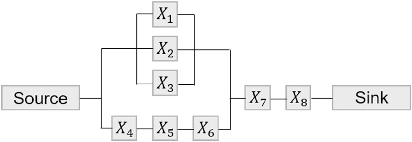
We use the example reliability block diagram illustrated below, used in Byun et al. (2019).

The network consists of 8 components $X_1, \cdots, X_8$, which take a binary-state, 0 for failure and 1 for survival.
Their probability distributions are set to $P(X_i=0) = 0.1$ and $P(X_i=1) = 0.9$, $n=1,\cdots,8$.
The component probabilities are statistically independent.
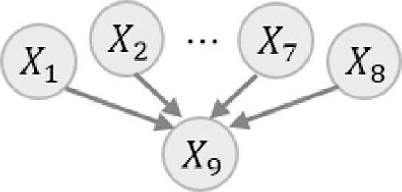
The system’s state is represented by a random variable $X_9$, whose failure is defined by the disconnection between the source and the sink.
This relationship leads to the BN graph below.

For decision-making, we are interested in (1) system failure probability and (2) component importance measure.
For more technical details about Bayesian network, matrix-based Bayesian network, or the example, please refer to Byun et al. (2019) and/or Byun and Song (2021).
Byun, J. E., Zwirglmaier, K., Straub, D. & Song, J. (2019). Matrix-based Bayesian Network for efficient memory storage and flexible inference. Reliability Engineering & System Safety, 185, 533-545.
Byun, J. E. & Song, J. (2021). Generalized matrix-based Bayesian network for multi-state systems. Reliability Engineering & System Safety, 211, 107468.
Quantification of probability distributions
Variable
There are two essential classes to quantify a BN: (1) variables and (2) CPMs (conditional probability matrices).
First, we need to define each variable by its name and the descriptions of its state.
varis = {}
varis['x1'] = variable.Variable(name = 'x1', values=['f', 's'])
Above, we created a dictionary varis to store all varables of the model.
As a starter, we defined the first component $X_1$.
The values must be a list that contains the description of each corresponding state.
As Python starts index from 0, above means that state 0 corresponds to f(ailure) and 1 to s(urvival).
The values list has two purposes.
First, MBNPy uses the list’s length to infer the total number of states to perform inferences.
Second, the descriptions serve as a reminder of what each state means for future reference or other users.
As all component have the same values, we repeat the same process for other components below.
n_comp = 8 # number of components
for i in range(1, n_comp):
    varis['x'+str(i+1)] = variable.Variable(name = 'x'+str(i+1), values=['f', 's'])

print(varis['x8'])
"Variable(name=x8, B=[{0}, {1}, {0, 1}], values=['f', 's'])"
For the system, the variable is also similar.
varis['x9'] = variable.Variable(name = 'x9', values=['f', 's'])
CPM
Now we define CPM (conditional probability matrix), which represents probability distribution.
We note that to quantify a BN, a probability distribution needs to be assigned to each node, being conditional on the corresponding node’s parent nodes.
Components
The components do not have any parent node as presented in the BN above.
Thus, their distributions are defined as a marginal distribution $P(X_i)$, $i=1,\cdots,8$.
We start from $X_1$.
cpms = {}
cpms['x1'] = cpm.Cpm(variables=[varis['x1']], no_child = 1, C=np.array([[0], [1]]), p=np.array([0.1, 0.9]))
Above, variables is a list of variables that constitute the distribution. In this case, there is only one variable involved.
no_child is the number of child nodes.
For instance, if there is a probability distribution $P(X_2,X_3 | X_1)$, one may set variables=[varis[‘x2’], varis[‘x3’], varis[‘x1]] and no_child=2.
In other words, no_child lets MBNPy know where to put the conditional bar.
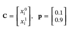
Event matrix C and probability vector p go together.
Each row of the two matrices refer to the same state, where C indicates what the state is and p indicates what the probability is.
In this case, they are defined as

where the figure has been brought from Byun et al. (2019).
More information is referred to Byun et al. (2019) and/or Byun and Song (2021).
We repeat the same quantification for other components.
for i in range(1, n_comp):
    cpms['x'+str(i+1)] = cpm.Cpm(variables=[varis['x'+str(i+1)]], no_child = 1, C=np.array([[0], [1]]), p=np.array([0.1, 0.9]))

print(cpms['x8'])
Cpm(variables=['x8'], no_child=1, C=[[0]
 [1]], p=[[0.1]
 [0.9]]
System
This is where MBNPy becomes different from other BN solutions.
MBNPy encodes a system’s distribution to reduce compuational cost.
Again, for more information, please refer to the references.
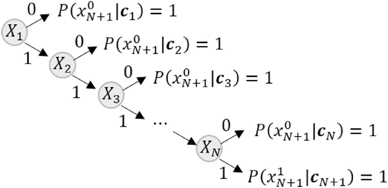
In Byun et al. (2019), a branch and bound algorithm (a system reliability method) is run as below:

Then, each branch can be represented by a row of C and p.
For instance, the upper most branch indicates the system fails when $X_8=0$ regardless of other components’ states.
Then, the probability distribution $P(X_9 | X_1,\cdots,X_8)$ has a row as below.
Csys = np.array([[0, 2, 2, 2, 2, 2, 2, 2, 0]])
psys = np.array([[1.0]])
Above, each column of Csys represents $X_9$ and $X_1,\cdots,X_8$ in order.
Note that the last element that represents $X_8$ is set to 0.
For other components, whose state does not matter in this instance, are set to a composite state 2 that can be either 0 or 1.
Given that there are two states 0 and 1 (from the values list of a Variable), MBNPy automoatically creates such composite state 2.
If given three states 0, 1, and 2, MBNPy creates composite state as 3 for 0 and 1, 4 for 0 and 2, 5 for 1 and 2, and 6 for 0, 1, and 2.
We hope this provides an idea of the pattern that MBNPy creates composite states.
The information about composite states is stored in B matrix (Byun and Song 2021).
For instance, let’s have a look at $X_1$’s B matrix:
print(varis['x1'].B)
[{0}, {1}, {0, 1}]
Now, we can create the C matrix consisting of the nine branches as follows.
Note that the p matrix also needs to have nine rows, whose values are all 1 as the system definition is deterministic so all conditional events happen with a probability of 1.
Note that while MBNPy needs only 9 rows, there are originally $2^{(8+1)}=512$ events to quantify.
Csys = np.array([[0, 2, 2, 2, 2, 2, 2, 2, 0],
                 [0, 2, 2, 2, 2, 2, 2, 0, 1],
                 [1, 1, 2, 2, 2, 2, 2, 1, 1],
                 [1, 0, 1, 2, 2, 2, 2, 1, 1],
                 [1, 0, 0, 1, 2, 2, 2, 1, 1],
                 [0, 0, 0, 0, 0, 2, 2, 1, 1],
                 [0, 0, 0, 0, 1, 0, 2, 1, 1],
                 [0, 0, 0, 0, 1, 1, 0, 1, 1],
                 [1, 0, 0, 0, 1, 1, 1, 1, 1]])
psys = np.array([[1.0]*9]).T

cpms['x9'] = cpm.Cpm(variables=[varis['x9'], varis['x1'], varis['x2'], varis['x3'], varis['x4'],
                                varis['x5'], varis['x6'], varis['x7'], varis['x8']],
                                no_child = 1, C=Csys, p=psys)

print(cpms['x9'])
Cpm(variables=['x9', 'x1', 'x2', 'x3', 'x4', 'x5', 'x6', 'x7', 'x8'], no_child=1, C=[[0 2 2 2 2 2 2 2 0]
 [0 2 2 2 2 2 2 0 1]
 [1 1 2 2 2 2 2 1 1]
 [1 0 1 2 2 2 2 1 1]
 [1 0 0 1 2 2 2 1 1]
 [0 0 0 0 0 2 2 1 1]
 [0 0 0 0 1 0 2 1 1]
 [0 0 0 0 1 1 0 1 1]
 [1 0 0 0 1 1 1 1 1]], p=[[1.]
 [1.]
 [1.]
 [1.]
 [1.]
 [1.]
 [1.]
 [1.]
 [1.]]
System risk assessment
Now we are ready to perform analysis. We can compute the system’s marginal distribution $P(X_9)$ by eliminating components.
cpm_sys = operation.variable_elim(cpms, [varis['x1'], varis['x2'], varis['x3'], varis['x4'],
                                         varis['x5'], varis['x6'], varis['x7'], varis['x8']])

print(cpm_sys)
print(f'System failure probability: {cpm_sys.p[0][0]:1.2f}')
Cpm(variables=['x9'], no_child=1, C=[[0]
 [1]], p=[[0.19021951]
 [0.80978049]]
System failure probability: 0.19
We can also compute component importance measure $P(X_i=0|X_9=0) = P(X_i=0,X_9=0) / P(X_9=0)$.
For instance, for $X_1$:
cpm_sys_x1 = operation.variable_elim(cpms, [varis['x2'], varis['x3'], varis['x4'],
                                            varis['x5'], varis['x6'], varis['x7'], varis['x8']])

print(cpm_sys_x1)

prob_s0_x0 = cpm_sys_x1.get_prob(['x1', 'x9'], [0,0])
print(f'P(X1=0 | X9=0): {prob_s0_x0 / cpm_sys.p[0][0]:1.2f}')
Cpm(variables=['x1', 'x9'], no_child=2, C=[[0 0]
 [0 0]
 [1 0]
 [0 1]
 [1 1]], p=[[2.195100e-04]
 [1.900000e-02]
 [1.710000e-01]
 [8.078049e-02]
 [7.290000e-01]]
P(X1=0 | X9=0): 0.10
We can repeat the process for all components:
CIMs = {} # component importance measures
for i in range(n_comp):
    varis_elim = [varis['x'+str(j+1)] for j in range(n_comp) if j != i]
    cpm_sys_xi = operation.variable_elim(cpms, varis_elim)

    prob_s0_x0 = cpm_sys_xi.get_prob(['x'+str(i+1), 'x9'], [0,0])
    CIMs['x'+str(i+1)] = prob_s0_x0 / cpm_sys.p[0][0]

print(CIMs)
{'x1': 0.10103858431766545, 'x2': 0.10103858431766545, 'x3': 0.10103858431766545, 'x4': 0.10031042557096277, 'x5': 0.10031042557096279, 'x6': 0.10031042557096273, 'x7': 0.5257084302235875, 'x8': 0.5257084302235875}
%matplotlib inline

plt.figure(figsize=(6, 3))
plt.bar(list(CIMs.keys()), list(CIMs.values()), color='skyblue')

# Add title and labels
plt.xlabel('Components')
plt.ylabel('CIMs')

# Show the plot
plt.show()

The results above show that $X_7$ and $X_8$ most critically affect the system’s failure.